ドップラー効果
周波数の関係式
| |
計測側が計測した周波数 |
| |
音速や光速など |
| |
観測者など計測側の移動速度 |
| |
音源など発生源の移動速度 |
| |
発生源が発生させた周波数 |
例: ベルトコンベアを連続して流れる箱の数
- 床面に固定され、十分な長さがある直線状のベルトコンベアがある
- ベルトと平行に移動しながらベルト上に箱を投入できる、移動可能な投入装置Sがある
- ベルトで運ばれて通過する箱の個数を計測できる、移動可能な計測装置Oがある
| ベルトが進む速度 | Va [m/秒] |
| 投入装置Sの移動速度 | Vs [m/秒] |
| 投入装置Sが投入する個数 | Ns [個/秒] |
| 計測装置Oの移動速度 | Vo [m/秒] |
| 計測装置Oが計測する個数 | No [個/秒] |
- 箱の寸法は十分に小さいものとし、箱の寸法は考慮しない
- 箱が投入される時間の間隔は全て均等とする
- ベルトが進む速度 Va は、投入装置Sの移動速度 Vs および計測装置Oの移動速度 Vo よりも速い
投入装置Sと計測装置Oの両方が床面に固定されている場合
時間が十分に経過した後における1秒間の動きを考える
| 箱同士の間隔 | Va/Ns [m] |
| 計測装置Oを1秒間に通過するベルトの長さ | Va [m] |
| ベルト上で長さ Va [m] 内にある箱の個数 | No [個] |
No[個] : Va[m] =  1[個] : (Va/Ns)[m]
               = Ns[個] :      Va[m]
No = Ns
投入装置Sだけが移動する場合
時間が十分に経過した後における1秒間の動きを考える
| 投入装置Sから見たベルトの進む速度 | Va-Vs [m/秒] |
| 箱同士の間隔 | (Va-Vs)/Ns [m] |
| 計測装置Oを1秒間に通過するベルトの長さ | Va [m] |
| ベルト上で長さ Va [m] 内にある箱の個数 | No [個] |
No[個] : Va[m] = 1[個]  : (Va-Vs)/Ns[m]
               = Ns[個] : Va-Vs[m]
No = (Va/(Va-Vs)) * Ns
計測装置Oだけが移動する場合
時間が十分に経過した後における1秒間の動きを考える
| 計測装置Oから見たベルトの進む速度 | Va-Vo [m/秒] |
| 箱同士の間隔 | Va/Ns [m] |
| 計測装置Oを1秒間に通過するベルトの長さ | Va-Vo [m] |
| ベルト上で長さ Va-Vo [m] 内にある箱の個数 | No [個] |
No[個] : Va-Vo[m] = 1[個]  : Va/Ns[m]
                  = Ns[個] : Va[m]
No = ((Va-Vo)/Va) * Ns
投入装置Sと計測装置Oの両方が移動する場合
時間が十分に経過した後における1秒間の動きを考える
| 箱同士の間隔 | (Va-Vs)/Ns [m] |
| 計測装置Oを1秒間に通過するベルトの長さ | Va-Vo [m] |
| ベルト上で Va-Vo [m] 内にある箱の個数 | No [個] |
No[個] : Va-Vo[m] = 1[個]  : (Va-Vs)/Ns[m]
                  = Ns[個] : Va-Vs[m]
No = ((Va-Vo)/(Va-Vs)) * Ns
例: ベルトコンベアを単発で流れる一連の箱
計測装置Oから十分に離れた場所でベルト上に一定数の箱を投入する場合を考える
| ベルトが進む速度 | Va [m/秒] |
| 投入装置Sの移動速度 | Vs [m/秒] |
| 投入装置Sが投入する個数 | Ns [個/秒] |
| 投入を継続する時間 | Ds [秒] |
| 計測装置Oの移動速度 | Vo [m/秒] |
| 計測を継続した時間 | Do [秒] |
| 投入装置Sから見たベルトの進む速度 | Va-Vs [m/秒] |
| 計測装置Oから見たベルトの進む速度 | Va-Vo [m/秒] |
- 投入装置Sによって { (Va-Vs)[m/秒] * Ds[秒] } のベルト区間に箱が { Ns[個/秒] * Ds[秒] } だけ投入された
- 投入装置Sで投入された一連の箱が十分に時間が経過した後、計測装置Oへ到着した
- 計測装置Oで一連の箱 { Ns * Ds } [個] を計測するのに { (Va-Vo)[m/秒] * Do[秒] } のベルト区間を計測した
ベルト区間は投入側と計測側で同じであるため
(Va-Vs)[m/秒] * Ds[秒] = (Va-Vo)[m/秒] * Do[秒]
(1/Do) = ((Va-Vo)/(Va-Vs)) * (1/Ds)
球の表面積
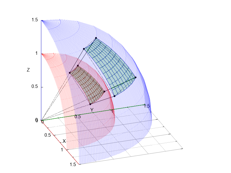
球面の座標
関数の近似
各点の位置関係
位置関係の近似
面積
# gnuplot 6.0 patchlevel 4

# 点の名称は便宜的に付けたものなので
# 他の資料における点の名称とは無関係

unset border
set xyplane at 0
set xzeroaxis linetype -1 linewidth 1.5 linecolor rgbcolor "0xC00000"
set yzeroaxis linetype -1 linewidth 1.5 linecolor rgbcolor "0x008000"
set zzeroaxis linetype -1 linewidth 1.5 linecolor rgbcolor "0x0000C0"
set grid xtics ytics mxtics mytics \
  linetype -1 linewidth 1 linecolor rgbcolor "0xA0A0A0", \
  linetype  0 linewidth 1 linecolor rgbcolor "0xA0A0A0"
set xtics axis 0.5
set ytics axis 0.5
set ztics axis 0.5
set mxtics 2
set mytics 2
set xlabel "X" offset 0
set ylabel "Y" offset 0
set zlabel "Z" offset 0, 0

$ptA_r00to10_xy30_zxy60 << EOD
0 0 0
0.75 0.433012702 0.5
EOD

$ptB_r10to15_xy30_zxy60 << EOD
0.75 0.433012702 0.5
1.125 0.649519053 0.75
EOD

$ptC_r00to10_xy30_zxy30 << EOD
0 0 0
0.433012702 0.25 0.866025404
EOD

$ptD_r10to15_xy30_zxy30 << EOD
0.433012702 0.25 0.866025404
0.649519053 0.375 1.299038106
EOD

$ptE_r00to10_xy60_zxy60 << EOD
0 0 0
0.433012702 0.75 0.5
EOD

$ptF_r10to15_xy60_zxy60 << EOD
0.433012702 0.75 0.5
0.649519053 1.125 0.75
EOD

$ptG_r00to10_xy60_zxy30 << EOD
0 0 0
0.25 0.433012702 0.866025404
EOD

$ptH_r10to15_xy60_zxy30 << EOD
0.25 0.433012702 0.866025404
0.375 0.649519053 1.299038106
EOD

$ptAtoC << EOD
0.75 0.433012702 0.5
0.433012702 0.25 0.866025404
EOD

$ptAtoE << EOD
0.75 0.433012702 0.5
0.433012702 0.75 0.5
EOD

$ptGtoC << EOD
0.25 0.433012702 0.866025404
0.433012702 0.25 0.866025404
EOD

$ptGtoE << EOD
0.25 0.433012702 0.866025404
0.433012702 0.75 0.5
EOD

$ptBtoD << EOD
1.125 0.649519053 0.75
0.649519053 0.375 1.299038106
EOD

$ptBtoF << EOD
1.125 0.649519053 0.75
0.649519053 1.125 0.75
EOD

$ptHtoD << EOD
0.375 0.649519053 1.299038106
0.649519053 0.375 1.299038106
EOD

$ptHtoF << EOD
0.375 0.649519053 1.299038106
0.649519053 1.125 0.75
EOD

set margins 0, 0, 0, 0
set view 65, 70, 1
set isotropic
set pm3d scansautomatic

unset colorbox
unset key

set parametric
set urange [pi/6:pi/3]
set vrange [pi/6:pi/3]
set xrange [0:1.5]
set yrange [0:1.5]
set zrange [0:1.5]

set isosamples 10
set samples 100

splot \
  1*sin(v)*cos(u),   1*sin(v)*sin(u),   1*cos(v) with lines linecolor rgbcolor "0xC00000", \
  1*sin(v)*cos(u),   1*sin(v)*sin(u),   1*cos(v) with pm3d  fillstyle transparent solid 0.1 fillcolor rgbcolor "0x00C000", \
1.5*sin(v)*cos(u), 1.5*sin(v)*sin(u), 1.5*cos(v) with lines linecolor rgbcolor "0x0000C0", \
1.5*sin(v)*cos(u), 1.5*sin(v)*sin(u), 1.5*cos(v) with pm3d  fillstyle transparent solid 0.1 fillcolor rgbcolor "0x00C000", \
$ptA_r00to10_xy30_zxy60 with linespoints linetype  0 linewidth 1.5 linecolor rgbcolor "0x000000", \
$ptB_r10to15_xy30_zxy60 with linespoints linetype -1 linewidth 1.5 linecolor rgbcolor "0x000000" pointtype 7 pointsize 1, \
$ptC_r00to10_xy30_zxy30 with linespoints linetype  0 linewidth 1.5 linecolor rgbcolor "0x000000", \
$ptD_r10to15_xy30_zxy30 with linespoints linetype -1 linewidth 1.5 linecolor rgbcolor "0x000000" pointtype 7 pointsize 1, \
$ptE_r00to10_xy60_zxy60 with linespoints linetype  0 linewidth 1.5 linecolor rgbcolor "0x000000", \
$ptF_r10to15_xy60_zxy60 with linespoints linetype -1 linewidth 1.5 linecolor rgbcolor "0x000000" pointtype 7 pointsize 1, \
$ptG_r00to10_xy60_zxy30 with linespoints linetype  0 linewidth 1.5 linecolor rgbcolor "0x000000", \
$ptH_r10to15_xy60_zxy30 with linespoints linetype -1 linewidth 1.5 linecolor rgbcolor "0x000000" pointtype 7 pointsize 1, \
$ptAtoC with lines linetype 0 linewidth 1.5 linecolor rgbcolor "0x000000", \
$ptAtoE with lines linetype 0 linewidth 1.5 linecolor rgbcolor "0x000000", \
$ptGtoC with lines linetype 0 linewidth 1.5 linecolor rgbcolor "0x000000", \
$ptGtoE with lines linetype 0 linewidth 1.5 linecolor rgbcolor "0x000000", \
$ptBtoD with lines linetype 0 linewidth 1.5 linecolor rgbcolor "0x000000", \
$ptBtoF with lines linetype 0 linewidth 1.5 linecolor rgbcolor "0x000000", \
$ptHtoD with lines linetype 0 linewidth 1.5 linecolor rgbcolor "0x000000", \
$ptHtoF with lines linetype 0 linewidth 1.5 linecolor rgbcolor "0x000000", \
1*sin(3*(v-pi/6))*cos(3*(u-pi/6)), 1*sin(3*(v-pi/6))*sin(3*(u-pi/6)), 1*cos(3*(v-pi/6)) \
with pm3d fillstyle transparent solid 0.1 fillcolor rgbcolor "0xFF0000", \
1.5*sin(3*(v-pi/6))*cos(3*(u-pi/6)), 1.5*sin(3*(v-pi/6))*sin(3*(u-pi/6)), 1.5*cos(3*(v-pi/6)) \
with pm3d fillstyle transparent solid 0.1 fillcolor rgbcolor "0x0000FF"
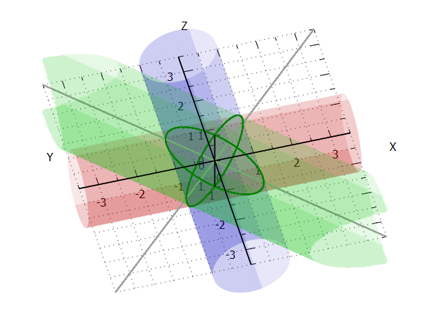
gnuplot 交差する円柱を描く
媒介変数を用いてsplotコマンドで円柱を描く
# gnuplot 6.0 patchlevel 4

unset border
set xyplane at 0
set xzeroaxis linetype -1 linewidth 1.5
set yzeroaxis linetype -1 linewidth 1.5
set zzeroaxis linetype -1 linewidth 1.5
set grid xtics ytics mxtics mytics linetype 0 linewidth 1.5
set xtics axis 1
set ytics axis 1
set ztics axis 1
set mxtics 2
set mytics 2
set xlabel "X" offset  30
set ylabel "Y" offset -30
set zlabel "Z" offset   0, 10

set margins 0, 0, 0, 0
set view 40, 345, 1.75
set isotropic
set pm3d scansautomatic

unset colorbox
unset key

set parametric
set urange [*:*]
set vrange [*:*]
set xrange [-3.5:3.5]
set yrange [-3.5:3.5]
set zrange [-1:1]

set isosamples 200
set samples 300

splot \
  u, \
  cos(v), \
  sin(v) \
  with pm3d fillstyle transparent solid 0.1 fillcolor rgbcolor "0xC00000", \
\
  cos(u), \
  v, \
  sin(u) \
  with pm3d fillstyle transparent solid 0.1 fillcolor rgbcolor "0x0000C0", \
\
  u, \
  u, \
  0 \
  with lines linetype -1 linewidth 1.5 linecolor rgbcolor "0xA0A0A0", \
\
  u, \
  -u, \
  0 \
  with lines linetype -1 linewidth 1.5 linecolor rgbcolor "0xA0A0A0", \
\
  (sqrt(2)*cos(u))*cos(pi/4) - (v)*sin(pi/4), \
  (sqrt(2)*cos(u))*sin(pi/4) + (v)*cos(pi/4), \
  sin(u) \
  with pm3d fillstyle transparent solid 0.1 fillcolor rgbcolor "0x00C000", \
\
  (sqrt(2)*cos(u))*cos(pi/4), \
  (sqrt(2)*cos(u))*sin(pi/4), \
  sin(u) \
  with lines linecolor rgbcolor "0x008000" linewidth 1.5, \
\
  (sqrt(2)*cos(u))*cos(pi/4), \
  -(sqrt(2)*cos(u))*sin(pi/4), \
  sin(u) \
  with lines linecolor rgbcolor "0x008000" linewidth 1.5
WebPファイルに保存
set terminal webp size 640, 480 notransparent noanimate
cd 'c:\tmp'
set output 'test.webp'
refresh
unset terminal
